Facebook Profile Data Analysis
It’s fun to see data about yourself. So upon learning that you can download all of your facebook data, I think it’s natural to want to analyze it.
Facebook makes it quite easy to download all of your data, but analyzing it is harder. You get a .zip file with a lot rather ugly html pages in it filled with everything you’ve done on facebook. It’s not conducive to seeing patterns or understanding your usage.
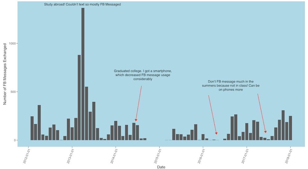
I decided to look at my facebook message history in R. Mostly I was interested in how my message frequency changed over time with specific people. It’s cool to see a graphical display of a relationship as it matures (and, sometimes, abruptly ends).
I’ll walk through how I went about the analysis, from downloading the data to creating the graphics.
Getting your data from Facebook
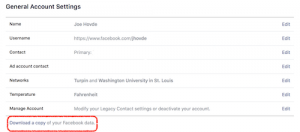
This is really easy. Navigate to facebook.com/settings and click on the link at the bottom. That’s it.

A zip archive with all of your activity will download. Explore this a bit to familiarize yourself with the data and to revisit wall posts from 8 years ago.
Reading the data into R
Now, I read the url of the “messages” section into R. A great resource for getting started with web / html scraping is from Hadley Wickham here.
Here’s the code I used for the analysis.. Please let me know (@jhovde2121 on twitter) if you have any questions or any suggestions on how this could be done in a better way.
Facebook Messages
library(dplyr)##
## Attaching package: 'dplyr'## The following objects are masked from 'package:stats':
##
## filter, lag## The following objects are masked from 'package:base':
##
## intersect, setdiff, setequal, unionlibrary(tidyr)
library(rvest)## Loading required package: xml2library(lubridate)##
## Attaching package: 'lubridate'## The following object is masked from 'package:base':
##
## datelibrary(ggplot2)Get the data: First, get the filepath of your message file. Then, choose which friend you want to analyze data with. I just used CTRL + F to find the friend and then used that file path (it so happens that this friend was number 691).
If you wanted to analyze all of your messages to everyone, you could loop through all of your friends and use that data instead.
url <- "facebook-jhovde-2018/html/messages.htm"
raw <- read_html(url)

# this is the list of people I had messages with
people <- raw %>%
  html_nodes("div.contents a") %>%
  html_text %>%
  data_frame()

# making html session

session <- html_session("file:///Users/josephhovde/RProjects/facebook-jhovde-2018/messages/691.html")

# iterating through them
friend <- read_html("facebook-jhovde-2018/messages/691.html")

# used the great SelectorGadget chrome plugin to find the html node I wanted ("span.meta")
friend_df <- friend %>%
  html_nodes("span.meta") %>%
  html_text() %>%
  data_frame()

# reformatting the dates. This takes some patience.

friend_df <- friend_df %>%
  rename(moment = ".")

friend_df <- friend_df %>%
  separate(moment, c("weekday", "monthday", "yeartime"), ",")

friend_df <- friend_df %>%
  separate(yeartime, c("year", "time"), "at")


# group by year

friend_df %>%
  group_by(year) %>%
  summarise(n = n()) %>%
  ggplot(aes(x = year, y = n)) +
  geom_col(aes(fill = year))
# group by day of week
friend_df %>%
group_by(weekday) %>%
summarise(n = n()) %>%
ggplot(aes(x = reorder(weekday, n), y = n)) +
geom_col(aes(fill = weekday))# trim exces whitespace
friend_df$time <- trimws(friend_df$time)
friend_df$monthday <- trimws(friend_df$monthday)
friend_df <- friend_df %>%
separate(time, c("time", "timezone"), " ")
# separate month and day of month
friend_df <- friend_df %>%
separate(monthday, c("month", "day"), " ")
# putting it in day month year
friend_df <- friend_df %>%
mutate(dmy = paste(day, month, year, sep = " "))
# getting the dates properly formatted. This was harder to figure out than it should have been
friend_df$dmy <- as_date(x = friend_df$dmy, format = "%d %B %Y")Now that I have the dates properly formatted, I do some analysis to check out the change of messages over time. I use the cut() function which can breka your dates into weeks, months etc; it was new to me and is very useful.
# This is a chart of number of messages per day. Can see patterns but it's too granular.

friend_df %>%
  group_by(dmy) %>%
  summarise(n = n()) %>%
  arrange(dmy) %>%
  ggplot(aes(x = dmy, y = n)) +
    geom_col()
# This cuts the data up by week. Very useful!
friend_df$week <- as.Date(cut(friend_df$dmy, breaks = "week"))
friend_df %>%
group_by(week) %>%
summarise(n = n()) %>%
arrange(week) %>%
ggplot(aes(x = week, y = n)) +
geom_col()# same thing, cutting by month
friend_df$month_cut <- as.Date(cut(friend_df$dmy, breaks = "month"))
# chart of monthly messages over time
friend_df %>%
group_by(month_cut) %>%
summarise(n = n()) %>%
arrange(month_cut) %>%
ggplot(aes(x = month_cut, y = n)) +
geom_col() +
scale_x_date(date_breaks = "1 year") +
labs(title = "Facebook Messages Exchanged Over Time",
subtitle = "With One Friend Since 2012",
x = "Date",
y = "Number of FB Messages Exchanged") +
theme(axis.text.x = element_text(angle = 70, hjust = 1),
panel.background = element_rect(fill = "lightblue"),
panel.grid.major = element_blank(),
panel.grid.minor = element_blank())
Thanks for reading! If you enjoy this type of analysis, follow me on twitter or sign up to be notified of new posts below.
